2024-11-03

Yo. This is the first note of the summer. Today I brushed off the last snaggles of exam fatigue and started thinking about how this summer is going to look.

• I'm planning on full sending it into mech interp projects / research (while keeping up with my math, etc). Four months is a long time, and right now I feel like I have all the time in the world, but I know it's going to go quicker than anything. Hopefully I can document as much as possible... 'artifact' generation seems to be the only way to tie yourself down when everything around you moves this fast.

• I want to spend as little of these four months doing things manually where I could automate them, especially re Mech Interp stuff. As I go I want to automate as much of my research workflow as I can. Hopefully I can make some of this stuff public, but I'm not going to be trying to solve everyones workflow, just mine.

• I'm going to be trying to be more purposeful with my note taking - right now this looks like throwing any terms / formulas / concepts I don't understand into anki. I've used spaced repetition in the past (I decided it would be a good idea to take a biology class (it was not)). Hopefully this will make bringing ideas down into working memory for triangulation and cross-pollination easier.

I was busy until around 4pm today, but I managed to get through the transformer implementation section of the ARENA course

• hack up this 'daily post' stuff. Never used einops before but I'm hoping it's going to solve the broadcasting hell that pytorch always seems to be for me.

Here's my implementation of attention with einops (problem from the ARENA course):

def forward(
    self, normalized_resid_pre: Float[Tensor, "batch posn d_model"]
) -> Float[Tensor, "batch posn d_model"]:
 
    # leave b as is, leave q as is, mult and sum over d, leave h as is
    keys = t.einsum('bkd,ndh->bknh', normalized_resid_pre, self.W_K)
    queries = t.einsum('bqd,ndh->bqnh', normalized_resid_pre, self.W_Q)
    values = t.einsum('bvd,ndh->bvnh', normalized_resid_pre, self.W_V)
 
    keys, queries, values = keys+self.b_K, queries+self.b_Q, values+self.b_V
 
    # move q and k to the end, and dot product over the h, which is d_head
    # this gets the key x query matrix for each head
    attn_scores = t.einsum('bqnh,bknh->bnqk', queries, keys)
 
    # scale and apply mask
    masked = self.apply_causal_mask(attn_scores/self.cfg.d_head ** 0.5)
    attn_probs = t.softmax(masked, dim=-1)
 
    # not completely sure why we put q after b here and not at the end
    weighted_values = t.einsum('bnqk,bknh->bqnh', attn_probs, values)
 
    # linear map to get query results into the RS
    result = t.einsum('bqnh,nhe->bqne', weighted_values, self.W_O)
 
    # sum over all heads by omitting n in the result
    attn_output = t.einsum('bqne->bqe', result)
 
    return attn_output + self.b_O

This one was less tricky than I thought but einsum is still not completely obvious to me. I'm really looking forward to the rest of the course, so far everything has been super nicely structured, short feedbadck loops are so tasty.

2024-11-04

11:35 - finished chapter 1.1 from ARENA.

12:30 - reading https://www.lesswrong.com/posts/vJFdjigzmcXMhNTsx/simulators#The_limit_of_sequence_modeling

from the post:

In fact, [GPT-N] is not specifically optimized to give true answers, which a classical oracle should strive for, but rather to minimize the divergence between predictions and training examples, independent of truth

• I think the takeaway from this is that GPT-N would be able to predict the truth because somewhere deep down it's learned everything there is to know about the core generator function that is our universe; All the sentence continuations GPT is trained on are artifacts of our 'reality', no matter how fantastical and out of world any data may be. Even knowing the true distribution lies somewhere in the model, you'd have to actualy get the model to a place where you can sample the just the 'important truths' out of the world model, ignoring the 'unimportant truths' that are reflections of the input prompt.
• Janus put this much better than I could later in the post:

the upper bound of what can be learned from a dataset is not the most capable trajectory, but the conditional structure of the universe implicated by their sum (though it may not be trivial to extract that knowledge)

• Amazing foreshadowing of o1 here:

Or, in other words, the more general problem we have to solve is not asking GPT the question[20] that makes it output the right answer, but asking GPT the question that makes it output the right question (…) that makes it output the right answer.[21]

The post got me thinking about models that do cellular automata again. Ages ago I tried doing gradient ascent on GOL kernels so that they would lead to a desired board state after some num of timesteps but it didn't work very well as the gradients (with a differentiable update rule) from repeatedly updating the board state were super messy. I think I could try this again, I didn't really know what I was doing last time. I might try training a model to predict the start board state given a final board state as input, which I could do by either creating a dataset or trying to figure out an RL method. It would be sick to learn a general computation function (maybe from a dataset) and then see how 'weird' (OOD) you could make the target boards / how it scales, etc. The fun part would be having it learn the starting board for an arbitrary image and having the image 'assemble' + have it try fractals and space filling curves etc.

2:00 - started messing around with training a model to predict starting boards given an output board.

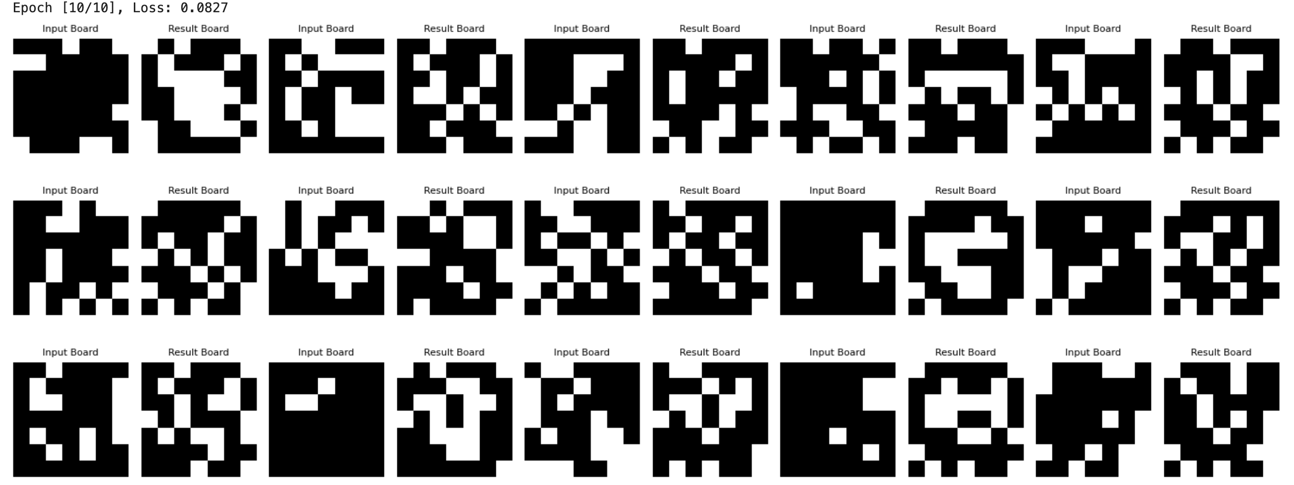
5:00 - simple 2 layer transformer seems to be training, for right now it's on a super simple dataset where it just has to predict the board one step back. I'm going to leave this training for a bit and try and keep going through ARENA on the colab. The data is basically given 3 as input predict 2 (or any other state which leads to 3 after a step):

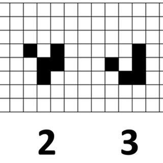
5:24 - Paused training because I realized that because there are multiple boards at step i-1 that lead to the same board at step i, the model could be correctly generating start boards but because we're training on input output pairs the model will get penalized even if it was right. duh.

5:50 - Modified the training loop to mask out all boards that correctly reproduce the start board when played for n steps, regardless of similarity to the target start board. So we're still using the target start board to update grad when incorrect. Not sure how this will affect learning, because a model being 'almost' correct will be penalized on a correct board that may be very different from it's prediction.

8:20 - Back from gym and dinner. Model still puffing along but I think I'm going to change up the loss function / increase learning rate here.

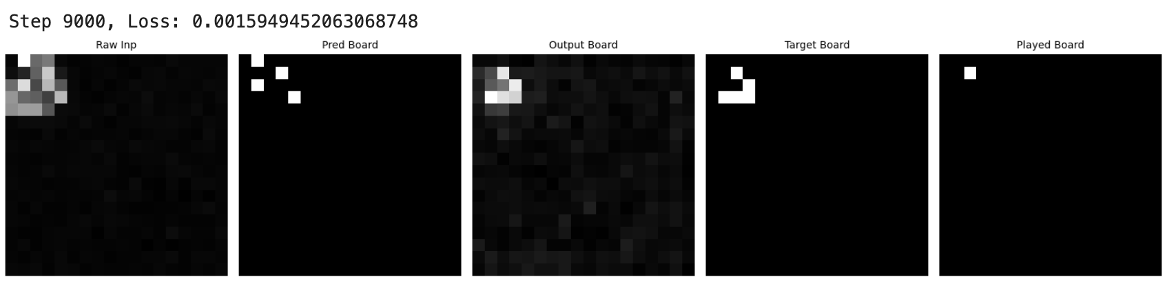
8:40 - Turns out the little tiny model (2 layer transformer, 256 d_model) was doing gods work on these outputs and definitely manages to lock down a vibe. Plot (at above loss) comparing result of running GOL update on models predicted previous state vs the input state:

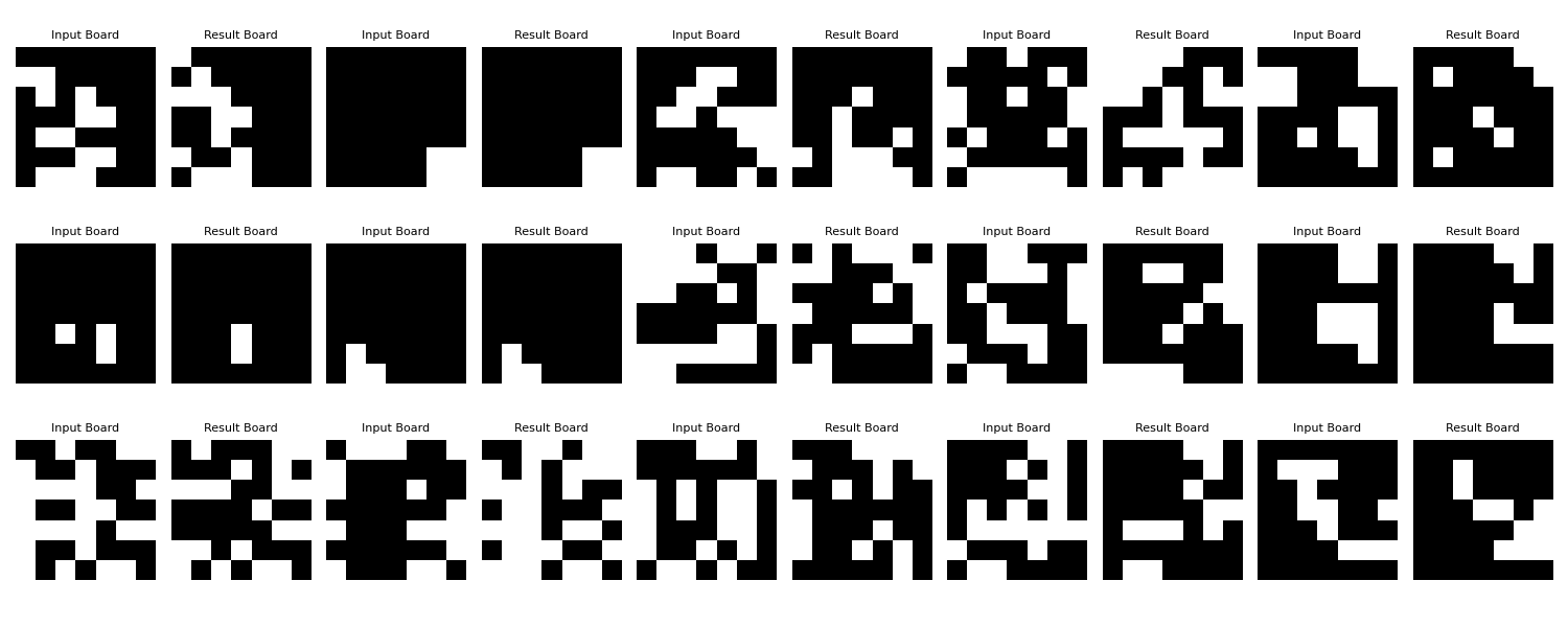
Going to leave a 3 layer 512-d johnny training while I do some more arena course.

10:27 - no comment

9:00 next day - I come back to training overnight and the loss is... weird. Accuracy is still terrible but I might just try being patient and letting it converge. I think the sawtooth is from batches + the training data forcing 'almost correct' answers to a completely different 'correct' answer.

2024-11-05

9:00 - Worked for a little while on the ARENA mech interp chapters while messing with the CA training. I got impatient with the model and paused it to try out training with differentiable update rules (done using sigmoid), but that didn't really work out super well, low loss but model was clearly not learning so something was wrong. Also tried some very poor RL where I would sample from the logits as actions and then try to use that in the loss function, but it didn't work at all (all this to get around non-differentiable update rules). I think just input/output pairs is the way to go, maybe a big enough dataset is all you need.

1:11 - Just finished up polishing the site so daily posts are all bundled together in one big scroll. All posts are concatenated into a huge MDX and rolled together. It makes the posts much more readable as work can flow over from one day to the next. Might change up the landing page to make it more homely.

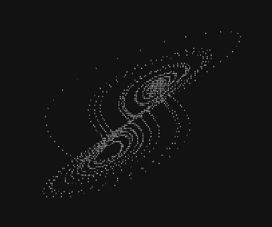
1->5:00 - improved the Lorentz attractor on the homepage so that it spins and has a variable resolution.

6->8:00 - went back to the model training and ended up scrapping the differentiable reversing. Seems like gradients just don't flow well even when using a very soft approximation of the update rules. Now I want to see if models trained to predict the next board can be run with gradient ascent to find an input board that leads to a target board. Probably wont work well, but it will be interesting to mess with L1 and other penalties as the problem is roughly like other many->one problems.

Anyways, turns out training models to calc forward like this gives quite nice grokking behaviour over different board sizes. Call it Conways Grok.

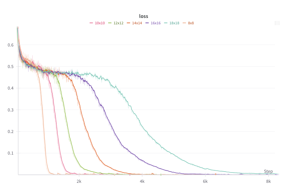
These models are accurate enough (>99.99%) to sample autoregressively. So we can run Conways with a model!

First two are on a slightly undertrained 12x12 model - the glider messes up at the end! Last is on a 18x18 model.

2024-11-06

Woke up tired as hell. Going to work on reversing the models + go back to just puffing through ARENA today. No more playing with react code.

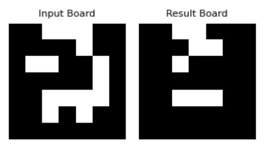
11:00 - First run at reversing the model via gradient ascent. Looking o.k. Going to try different input boards / optimizers / learning rates now.

board on left was the maxmimally activating input board - target output was the glider on the right, and in the middle is the result of running the input board

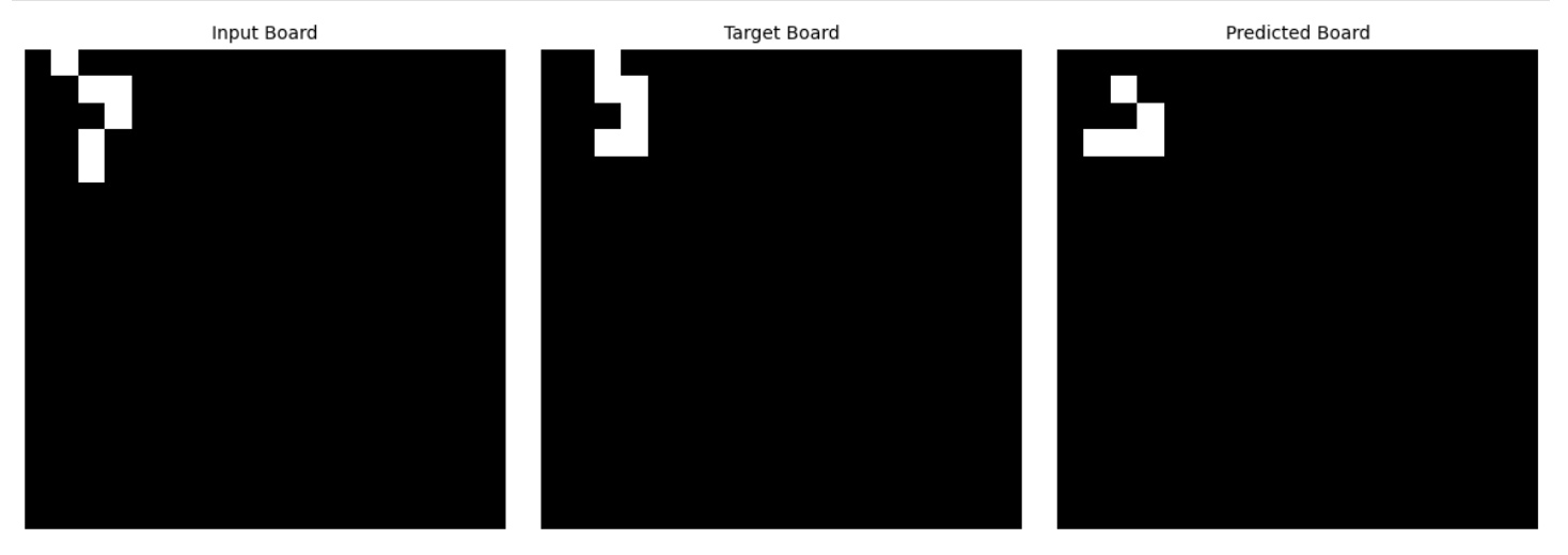
I'm thinking because going backwards is one->many, maybe I can just iteratively sample from the input dist to get something. Not sure if the model will converge to picking a single input.

Maximally activating, you can see we get continuous valued raw inputs which basically are the 'many' part of one->many. So when you threshold and play them they don't give the output, but when you run them through the model they do.

• tried sharp sigmoiding the inputs to get them roughly binary
  • didn't work
• tried using penaltys to force the values closer to either 0 or 1 + a a sparsity penalty

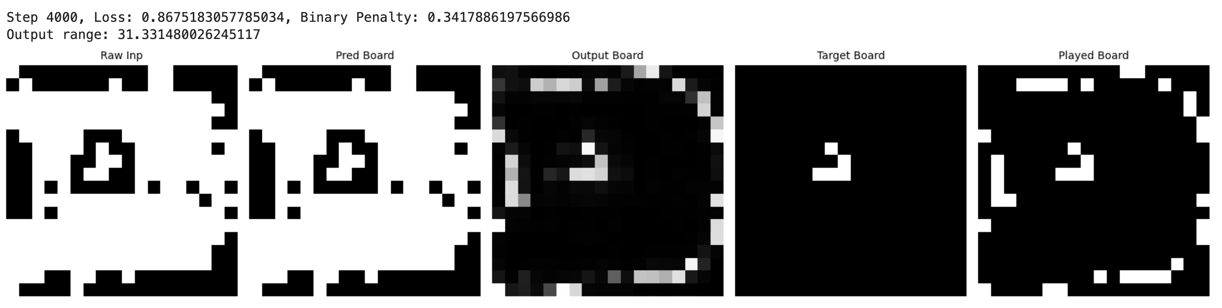
2:38 - Big progress!

Gradient ascent has worked to find a state that leads to the next glider step. Obviously sparsity needs to be improved but I think those are going to be fixable! Also, not 100% sure what's going on with the edges probably can be fixed padding the loss calc or something for future models. Very cool that such a complicated input maximally activates the model and is correct when played out!

Note to self - sparsity pen was 0.0 and binary pen was 0.3 direct on the outs

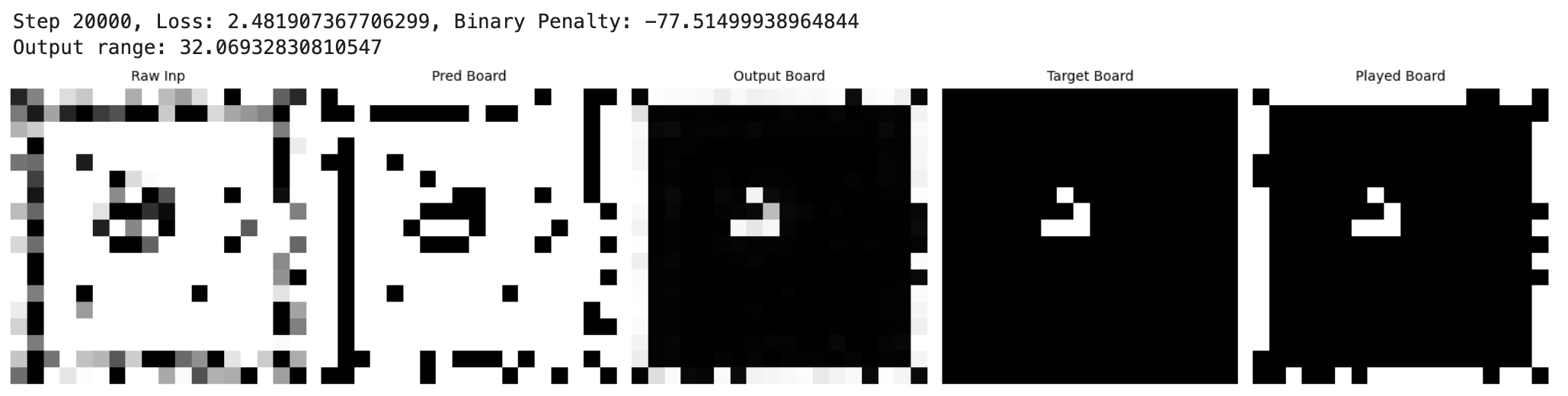
500 Binary pen on input_sigmoids

Maybe I could overcome some of my problems by making the model think in unit vectors? or something... Thinking about smushing a forward model into the training pass of the rev model. board -rev-> reversed -forward-> board. Anyways, I've gotten stalled with this for now, everything is too fiddly with hyperparams. I guess it's to be expected that a model wouldn't be able to do this.

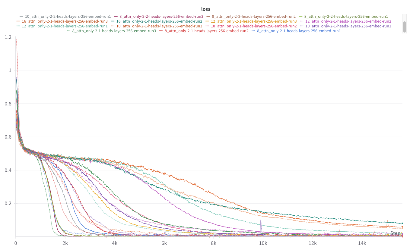
7:00 - Now I'm going to try and get a similar grokking chart as before but instead of board size increasing I'm going to increase num steps predicted. I think I need to chill out a bit and figure out how to actually do circuit analysis - these tasks seem perfect. We should be able to linearly probe out different board states on the multistep models, and hopefully find the circuits are the same. After I get the grokking chart for steps I'll try and train attention only versions.

2024-11-07

again tired.

9:15 - attention only models trained well overnight, now I have a bunch of models to mess with for after I do ARENA.

Seems like small boards can be solved with two layers + one head each, but a one layer couldn't solve shit and didn't exhibit the same grokking as the two layer models. Leaving this for now :).

Why doesn't wandb export your legend with the plot when you save it? Part of me wants to build my own pipeline lmao. Mech interp / ML research should be more like swimming through the mind of the machine. something cheap could be done now with codegen + better pipelines. Humans are going to need different interfaces as the value of low level thinking goes down. Maybe I just want pretty colors or something.

Time to do some math! I'm going to take another calc class towards the end of the summer, so I think I'll finish off lin alg on MA and then start calc2 asap. I want the class to be mostly revision by the time it rolls around.

3:00 - Put away the math. Got 2/3 of the way through the placement. even a week break from math makes problems tiring and slow.

4:22 - slightly golfed

def attn_detector(cache, match_fn):
    return [f"{layer}.{h}" for layer in [0, 1] 
            for h, head in enumerate(cache["pattern", layer]) if match_fn(head)]
 
current_attn_detector = lambda cache: attn_detector(cache, lambda h: h.diag().mean() > 0.4)
prev_attn_detector = lambda cache: attn_detector(cache, lambda h: h.diag(-1).mean() > 0.8)
first_attn_detector = lambda cache: attn_detector(cache, lambda h: h[:, 0].mean() > 0.8)
 
print("Heads attending to current token  = ", ", ".join(current_attn_detector(cache)))
print("Heads attending to previous token = ", ", ".join(prev_attn_detector(cache)))
print("Heads attending to first token    = ", ", ".join(first_attn_detector(cache)))

more golf

def generate_repeated_tokens(
    model: HookedTransformer, seq_len: int, batch: int = 1
) -> Int[Tensor, "batch full_seq_len"]:
    '''
    Generates a sequence of repeated random tokens
 
    Outputs are:
        rep_tokens: [batch, 1+2*seq_len]
    '''
    return t.tensor(
        [model.tokenizer.bos_token_id] + 
        [random.randint(0, model.cfg.d_vocab-1) for i in range(seq_len)]*2
      ).unsqueeze(0).to(device)

8:15 - gym, groceries, cleanup

9:35 - Finished the induction heads section of the mech interp intro chapter. still in awe resources like this exist. going to be up early, bedtime.

2024-11-08

Up on time. Did math from 7:15 -> 8:50, 9:00 -> 9:30, 9:45 -> 10:15 10:30 -> 11:00 revised anki + made some new cards

2:30, done some stuff. Thinking maybe It might not hurt to continue trying the training the reversible conways from dataset pairs, not completely sure why I stopped. It's a good toy model for asking the interesting question of how models can learn one->many functions.

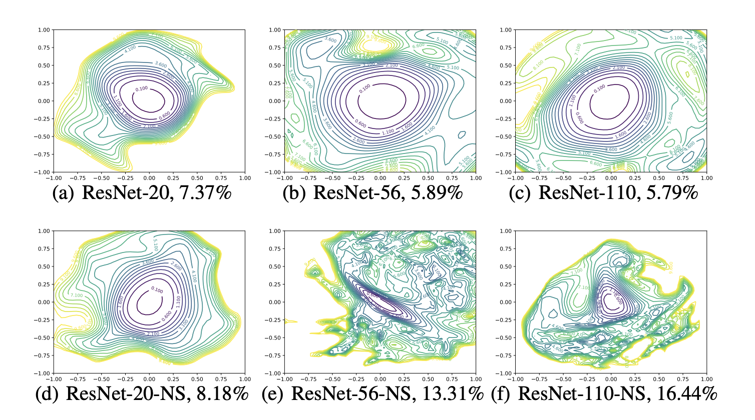
3:48 - Reading https://arxiv.org/pdf/1712.09913

• loss landscapes change with the model. This is seemingly obvious - the loss is parameterized not just by the problem but the model as well. Interesting to me that the glob min for two architectures trained on the same task could be the same, but everywhere else the loss could be different. When do two different models share a slice of a loss landscape given some translation? Is there any way to tell if two different models are going to implement the same solution? Could some quick and dirty measure of a landscapes complexity be used to run a model architecture search?

• What does using batch warmups make these look like?

It can be shown that the principle curvatures of a dimensionality reduced plot (with random Gaussian directions) are weighted averages of the principle curvatures of the full-dimensional surface

• my favourite thing about high dim vectors:

  It is well-known that two random vectors in a high dimensional space will be nearly orthogonal with high probability. In fact, the expected cosine similarity between Gaussian random vectors in n dimensions is roughly $\sqrt{2/(\pi n)}$

• Jesus... 'out of all parameter changes over training, which directions are the most explanatory'? I guess you could calculate partial covariance matrices or use partial SVDs on each batch or something to calc this

  Let θ_i denote model parameters at epoch i, and the final parameters after n epochs of training are denoted θn. Given n training epochs, we can apply PCA to the matrix M = [θ−θ_n; · · · ; θ_n−1 − θ_n], and then select the two most explanatory directions.

4:20 - back to ARENA. Some notes on induction circuits / attention circuits:

• attention outputs are just adding info to token slots in the residual stream - keys, queries, and values and are just transforms on each token slot
• This means if you want two tokens to attend to each other, you have to transform them into K's and Q's that are similar
• VK^TQ moves the value corresponding to whichever keys got "lit up" by the query into the residual stream just because similar keys and queries are high valued in K^TQ and others low valued
• this is basically a fuzzy dictionary - there will be noise in the atnn_output from KQ's that have slight overlap
• W_OV just takes a token, queries other tokens based on the head doing W_K(Resid_[token]), then writes their values to Resid_[token]

2024-11-09

Up @ 7:30, math from 8:00 -> 10:30 - \ groceries \ - 11:20 -> 12:20. I guess I got less done than I would have liked? Or maybe math just takes a really long time.

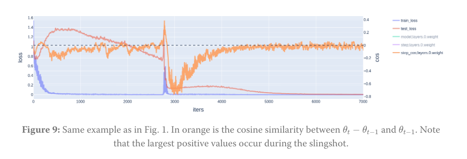
Reading: https://www.lesswrong.com/posts/LncYobrn3vRr7qkZW/the-slingshot-helps-with-learning

• They measure cosine similarity between parameter update steps, v interesting

  

• Your loss landscape will have a weight decay 'direction' and movement in parameter space will be driven by weight decay alone if loss is 0. When moving in the weight decay direction, eventually you'll hit a nonzero wall of loss, and you'll get a 'rebound' spike gradient update in the opposite direction, causing weight norm to shoot back up.

• No answer to why test loss goes down after slingshot. LLC goes down, meaning the model reaches a 'simpler' solution, but unsure why.

• this all happens because adamW momentum and variance all can get very small as you are just moving due to weight decay, and then when you hit an update you are basically moved just by the gradient, as your momentum and variance will be close to 0.

Now reading the official paper: https://openreview.net/forum?id=OZbn8ULouY

The norm grows rapidly sometime after the model has perfect classification accuracy on training data. A sharp phase transition then occurs in which the model misclassifies training samples. This phase change is accompanied by a sudden spike in training loss, and a deceleration in the norm growth of the final classification layer.

• Is this a phase change? In my head the term is reserved for models slowly building up small, independent circuits until they're able to merge them. But I guess 'phase change' might just encapsulate the changes in loss, norm, etc.

The features (pre-classification layer) show rapid evolution as the weight norm transitions from rapid growth phase to growth curtailment phase, and change relatively little at the norm growth phase.

2024-11-10

Day off. Read some papers.

2024-11-11

Math from 7:50 -> 12:30

Back to ARENA again today.

most useful diagram in the section, should have been much earlier IMO: https://raw.githubusercontent.com/callummcdougall/computational-thread-art/master/example_images/misc/composition_new.png

5:00, finished mech interp chapter 1.2

Important note by the big NN re toy models (I need to keep in mind - scientific method is not 'do something pretty' -> 'make up hypothesis after')

The right mindset for a toy model project is to take the process of setting up the toy model really seriously. Find something about a transformer that you're confused about, and try to distill it down to a toy model. Then try to red-team it, and think through ways it's disanalogous real models, and note down all of the assumptions you're making. (Easier to do with a friend! Outside perspectives are great) Then try to actually analyse the toy model, regularly keeping in mind the confusion about real models that you're trying to understand, and checking in on whether you've lost track. As you go deeper, you'll likely see ways the toy model could be more analogous, and can tweak the setup to be more true to the underlying confusion 'https://www.alignmentforum.org/posts/o6ptPu7arZrqRCxyz/200-cop-in-mi-exploring-polysemanticity-and-superposition'

2024-11-12

Math from 7:40 -> 9:50, got it done way quicker today.

Notes on arena / https://transformer-circuits.pub/2022/toy_model/index.html#demonstrating:

• They directly augment the importance of a feature by adding a coeff to the loss when calculating for a given feature

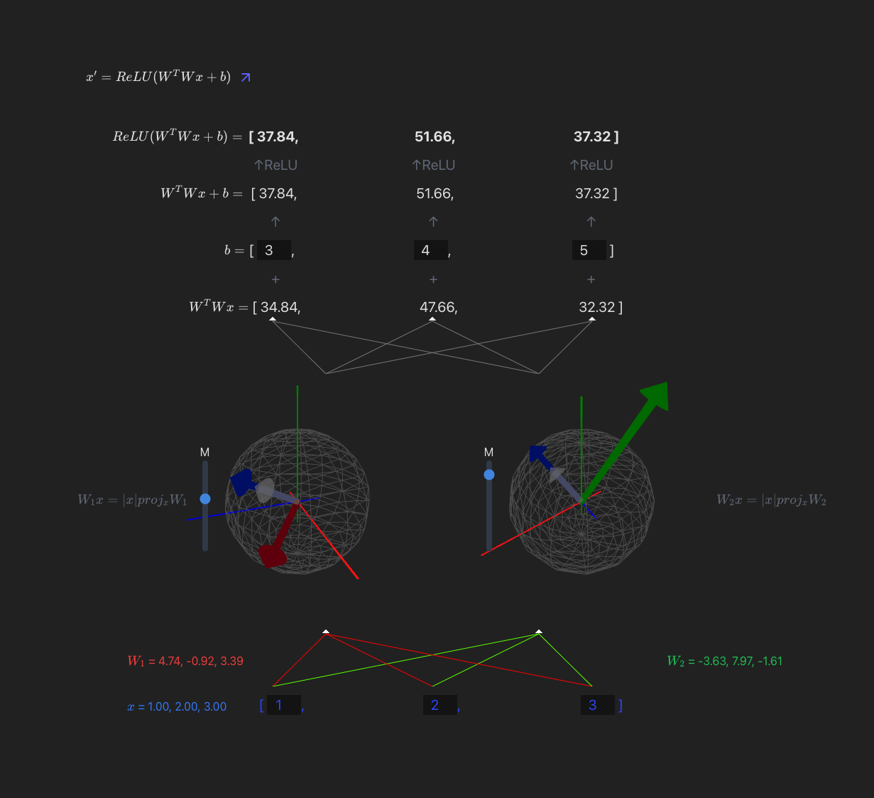
I want to make a widget that takes a model with 2 or 3 neurons in each hidden layer and visualizes the weight vectors for each neuron onto a circle/sphere, and then projects the prev layer activs in so you can visualize the dot product.

9:00 - something done! Following the model spec from TMOS. Because our input is 3d, we can represent each neurons input weights as a vector, and the input as another vector - (the output of a neuron is the dot product of these two). In this case the input is just input data, but if the model was multi-layer then you would have the activations of the last layer make up this 'feature' vector. Gif makes it look laggy unfortunately.

x' = ReLU(W^TWx + b)

11:00 - added a bias, controls for the magnitude, relu, visualization of the projection

I think this is a fun way to think about neurons which maybe gets overlooked a lot. Neurons basically just learn a vector and project their input onto it. Matrices can sometimes confuse people (like myself)

2024-11-13

11:30 - finished up the widget, going to eat and then do some math.

Widget is live @ https://max.v3rv.com/random/neuron-weight-projection-viz

Been a slow day, starting maths at 5:45... we'll see if I can get to arena or not did the math... phew

2024-11-14

7:45 -> coffee + math 10:45 -> done w math

3:51

there's something unique about writing code that just does shit to tensors, it really breaks you out of the for loop mindset

    def generate_anticorrelated_features(
        self, batch_size: int, n_anticorrelated_pairs: int
    ) -> Float[Tensor, "batch inst 2*n_anticorrelated_pairs"]:
        """
        Generates a batch of anti-correlated features. For each pair `batch[i, j, [2k, 2k+1]]`, each
        can only be non-zero if the other one is zero.
        """
        p = self.feature_probability[:, [0]]
        assert t.all(self.feature_probability == p)
        assert p.max().item() <= 0.5, "For anticorrelated features, must have 2p < 1"
    
        mags = t.rand(batch_size, self.cfg.n_inst, 2 * n_anticorrelated_pairs, device=p.device)
        one_pres = (t.rand(batch_size, self.cfg.n_inst, n_anticorrelated_pairs, device=p.device) <= 2 * p)
        pres = t.randint(0, 2, (batch_size, self.cfg.n_inst, 1), device=p.device).bool()
        
        mask = t.cat([pres, ~pres], dim=-1) * one_pres.repeat_interleave(2, dim=-1)
        return mags * mask

in the Lex/Dario/Amanda/Chris podcast Chris Olah said mentioned how the core idea of the superposition hypothesis is that models are simulating much higher dim models, and that it's likely gradient descent is actually navigating a much higher dimensional, sparse space, which it is learning to project down into our comparatively teeny matrices we give them. Compressed sensing allows us to recreate sparse, high dim matrices from dense, low dim projections - note to self to learn more @TODO. A big gap in my knowledge is this + information theory; even though I enjoy tickling myself with thoughts about 'bits' and 'entropy' etc etc I really couldn't have a clue.

Cool book - https://www.amazon.com.au/Introduction-Systems-Biology-Principles-Biological/dp/1584886420

Note to self on asymmetric superposition:

If a neuron represents some number of features in superposition, and it's weights for these features (assuming a toy model where inputs are features?) are asymmetric, meaning Wf1 $\gg$ Wf2 or Wf2 $\ll$ Wf1, then the model has chosen to allow one feature to heavily interfere with the other, but not the other way around. This is because even a small activation of f1 when Wf1 $\gg$ Wf2 will completely obliterate f2, but a little interference of f2 when f1 is present won't hurt f1. The 'output' weights (output weights? weird term) of the neuron can implement the reciprocal of W, so that large and small true activations of f1 and f2 are normalized, but this reciprocal normalization messes up when The issue is that if Wf1 and Wf2 are both significant, the reciprocal output weights fail to normalize and instead boost the norm. The model can then use a later neuron to inhibit this large positive activation by flipping it's sign and throwing it under the ReLU to dampen/chop it. This allows one feature to dominate or "mask" another + selectively tune which features are allowed to interfere.

8:00 -> Got sniped into TracR transformer compilation, want to train SAE's / do some other exps on these sparse models.

• Original Tracr paper: https://arxiv.org/pdf/2301.05062
• learning transformer programs: https://proceedings.neurips.cc/paper_files/paper/2023/file/995f693b73050f90977ed2828202645c-Paper-Conference.pdf
• looped transformers https://proceedings.mlr.press/v202/giannou23a/giannou23a.pdf
• automated circuit discovery for mech interp: https://arxiv.org/pdf/2304.14997
• original rasp paper: https://arxiv.org/pdf/2106.06981

Worries:

Tracr models are too simple to apply a SAE

• They are already overcomplete? what is the information density of a tracr program x, what is the mono-semantic limit of the model size for program x?
• Can we combine programs together? Might have to actually write rasp but oh well.
• read and write to resid with trained w^t, compressing features into superposition, then compare found features to the features found in the full dim, sparser model. But how can we quantify 'features' in the larger model?

10:30 -> first things first, train an encoder on the decompressed models to see what happens

As expected training is trivial, residual stream variation is tiny compared to real models (already v decomposed). Will have to investigate if we can even get anything feature-like into the enc when it is this sparse. I doubt sae's will help with anything when the model is already orthogonal etc.

2024-11-15

8:30 -> 11:20 coffee + math 11:30 lunch + code

Notebooks are cool until you restart and realize you've been using variables that don't exist anymore for the last 10 hours. Time to re-do all the runs...

Tracr sae scratchpad:

• SAE's work like normal on the decompressed models, not sure how to interpret their features though

• can we use the fact that we know what layer is doing to diff encoder acts on different layers?

• Here's a hist of firing frequncies on a larger d_mult model, works fine:

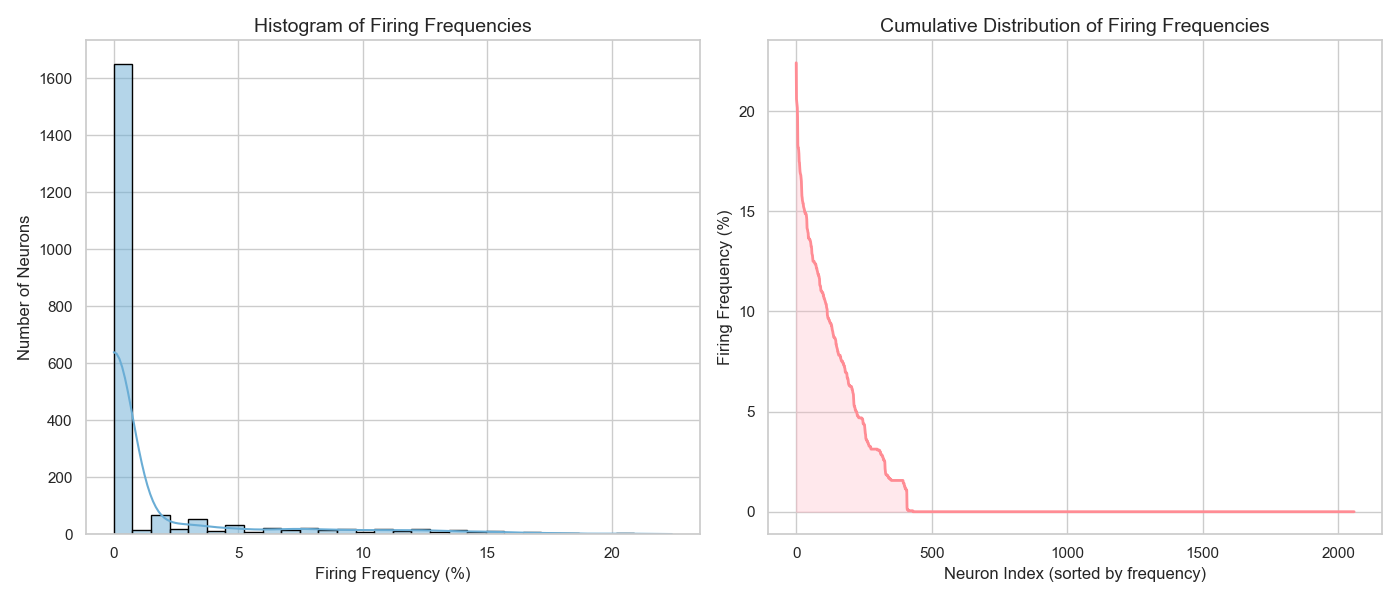
• Sparsity vs non-zero sae activation count over the dataset @ l1 = 0.1

• Same but at l1 = 1 and over 10 epochs per sae instead of 7

Back to the original paper:

We use a single linear projection W ∈ RD×d to compress the disentangled residual stream with size D to a smaller space with dimension d < D. We modify the model to apply WT whenever it reads from and W whenever it writes to the residual stream (see Figure 6). We freeze all other weights and train only W using stochastic gradient descent (SGD). Since vanilla Tracr models are sparse and have orthogonal features, this process can be viewed as learning the projection from a "hypothetical disentangled model" to the “observed model" described by Elhage et al. (2022b)

Ok. The Tracr models "are sparse and have orthogonal features" - We want to compress a tracr models residual stream, apply the sae, and find a method/metric for comparing the sae activations to the the decompressed residual streams 'true' features.

Seems to me that we don't need to 'freeze' the models weights and train the read/write W through the tracr model, we can just train the autoencoder directly on resid activs

Ok. Going through and replicating their training of the encoder on the sort task.

Maybe this is stupid. train an autoencoder to encode down, any 'sparse' autoencoder will just replicate the W^T? But the relu will just force the projection up to be different than W^T... Maybe some part of the SAE will not play nice with faithfully reconstructing the acts.

I think a next step might be to get a comparative performance analysis of SAE's trained on the same models compressed and regular residual streams.

• How many features does an sae on the compressed vs decompressed learn?
• Are these features similar?
• Can we find identical features?
  • cosine sim, manual inspection, etc
• what do the PCA of the two sae activs look like?

Quite similar, which is a nice sign:

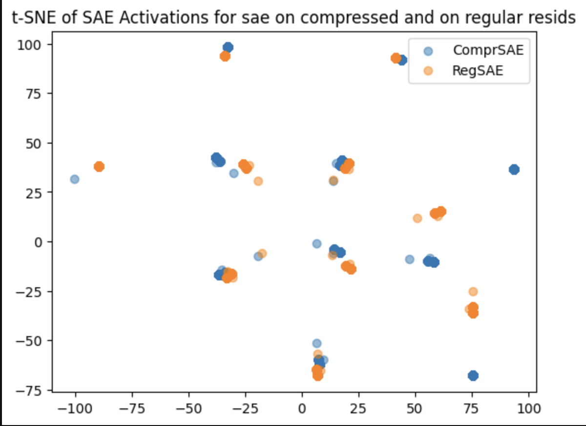
Number of significant singular values in the orthogonal residual stream is roughly = num features? So we take the cosine sim between the SAE feats and the PCA resid feats...

Activation sparsity for two same-size dictionary SAE's, one trained on the compressed residual stream and one on the regular, same l1 pen.

Regular Activatiosns Sparsity:  83.5981125
Compressed Activations Sparsity:  78.2952375, 
 
Regular Activations Sparsity:  75.8853125,
Compressed Activations Sparsity:  80.319125

Very high R^2 when training a linear transform between the two! Still with a 1:1 dictionary size

Mean Squared Error: 0.05293504521250725
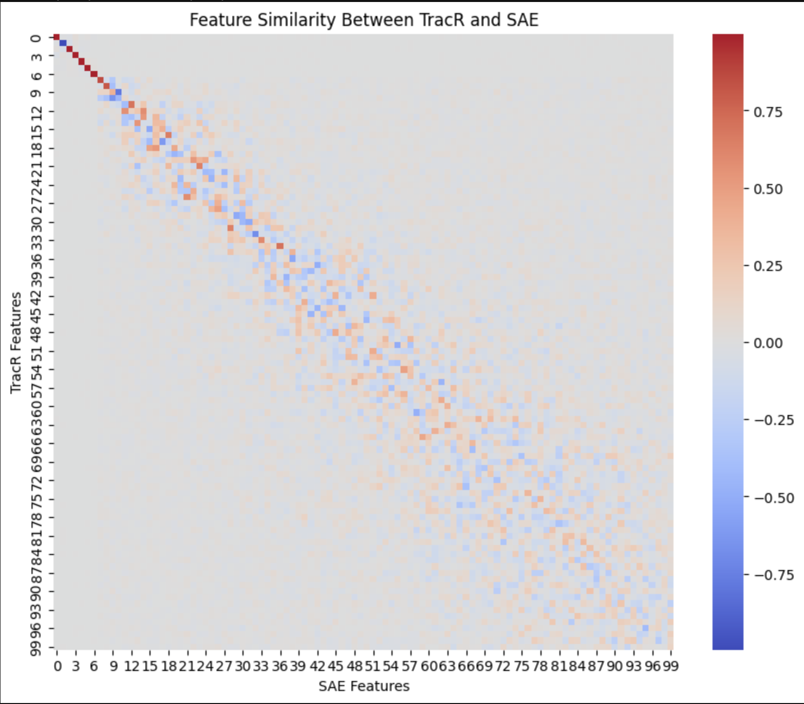
R^2 Score: 0.943285346031189

Cosine sim between the principal components of the transformed features from the 'compressed' SAE and the regular, d_mult=1:

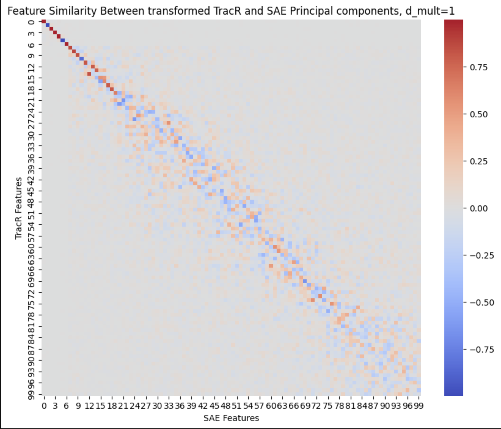
Finally getting somewhere nice.

The same but for SAE's with d_mult=2, we can see PC's are less aligned. Less variation in smaller solution spaces?

11:45 - Signing off, tomorrow I'm going to try and map those top 10ish principal components back to dataset examples for each, then finally compare this to what TracR is meant to be doing

2024-11-16

Skipped math and worked on tracr-sae's. Might update with findings soon

2024-11-17

Did extra math + a little bit of interp stuff, thought about things clearly for the first time in a while.

2024-11-18

Did Math, then coded up nice automated training sweep for a toy SAE trained on orthogonal data, will post results soon

2024-11-19

9:00 -> 12:30 Did lots of integrals.

Going to work on compiling down the data from the sweep and putting it into a little report, then hopefully back to more tracr stuff with the new data.

2024-11-20

8:30 -> 11:40 did lots of integrals

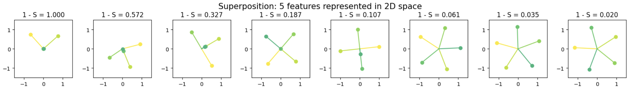
Today I want to take a break from training models and stuff and build a superposition geometry visualization widget, where you pass in a weight matrix and it isolates sections of features in superposition, and then calculates a possible geometry. Not completely sure on the math yet, but it should be something like converting the cosine sim to a distance, and then forcing the points to all conform to a set of distances (not sure how thats going to work yet). Then I can draw lines between points? or from the origin to the points, or something to represent shape. Maybe all points that share a dimension get an edge.

2024-11-25

Got back into it today! last couple days has been working on a small writeup + another superposition visualizer and just doing math like usual.

The writeup can be found here: https://max.v3rv.com/in-progress/saes-on-orthogonal-data

And the superpos thing can be found here: https://max.v3rv.com/random/superposition-viz

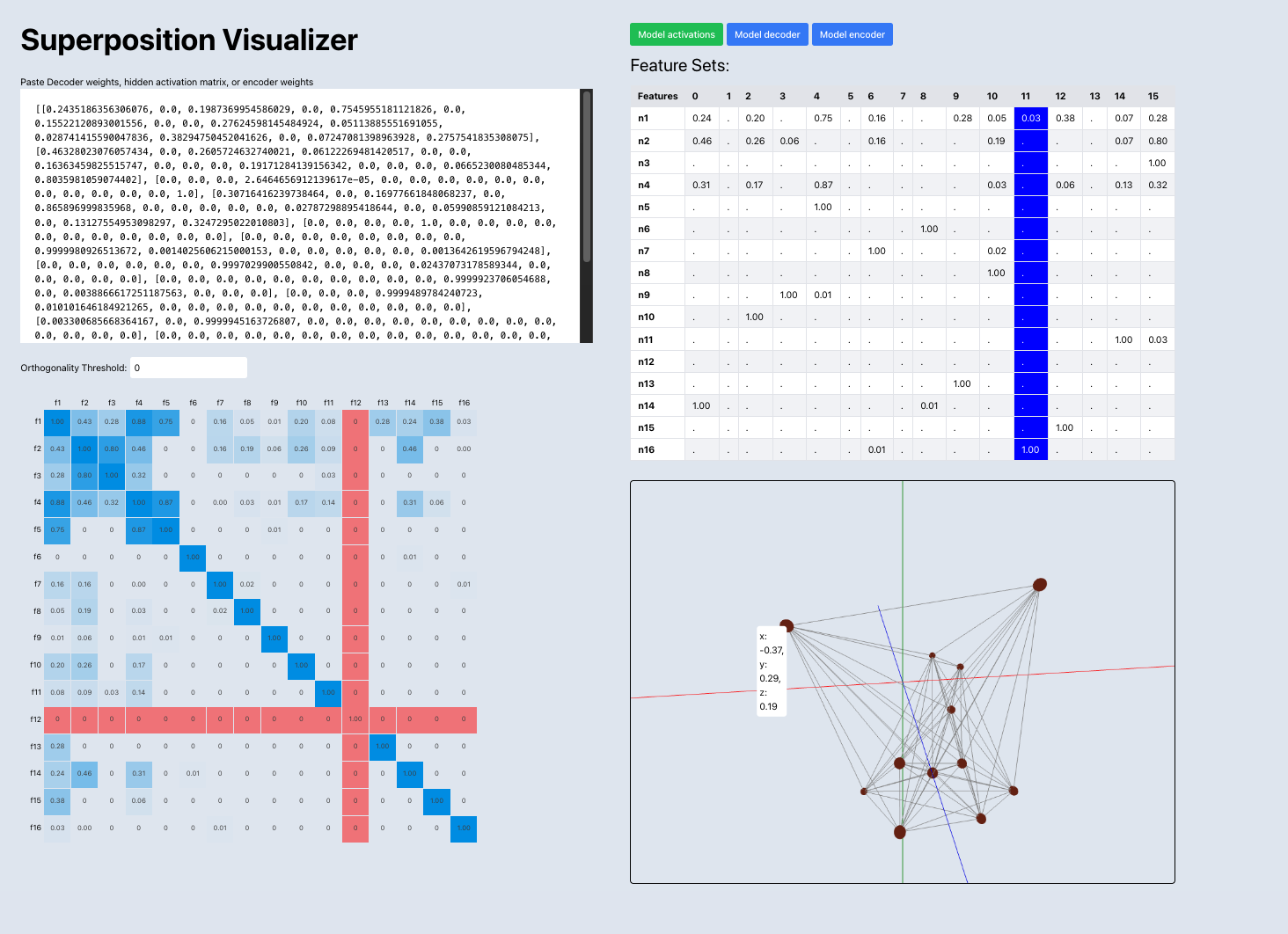
You might have to zoom out a bit for bigger models, my bad.

Also been thinking more about tracr models and SAE's trained on orthogonal data, here's a small writeup:

Starting to think about the big project - currently thinking about the relation of superpos/robustness, inspired by this tweet: https://twitter.com/livgorton/status/1849573082371064267.

Not really read on robustness stuff, so today I've just been going through some papers, notes dumped.

Adversarial Examples Are Not Bugs, They Are Features

Dataset level robustness

• Construct a robust dataset by training a robust model on the original, non spurious dataset, then gradient ascent to maximize used feature activation similarity on random input from said dataset. This adds spurious features to the real dataset, constructing a spurious dataset
• This basically removes the non-robust features from the dataset (the features that the robust model didn't use).
• You can improve robustness by training on a dataset that is robust
• Adversarial examples transfer between models because they arise from non-robust features
• PGD is a method of maximizing loss for a specific input while keeping within a similarity bound of the original image. This can be used to generate adversarial examples.
• Non robust features are shared between models because models all use spurious features to perform well - loss is correlated strongly with spurious feature transfer

Loss function level adversarial prevention

• loss is the maximum loss of any perturbed input in the valid set of perturbations

Learning from Incorrectly Labeled Data

• You can train a model, use it to generate incorrect labels on an OOD dataset or collect incorrect labels on in distribution examples into a new dataset, and then train a model on this new dataset - this model will recover performance on the original dataset because it has learned spurious correlations 'distilled' from the parent model - this is an example of feature distillation. "information about the trained model is being “leaked” into the dataset."

The Space of Transferable Adversarial Examples

• Fast Gradient Sign Method is good for 'finding multiple' adversarial directions, $\hat{x} = x +\epsilon \cdot \nabla_{x}sign(L(x, y))$. Can use a normalized L instead of sign for different norms
• Finds decision boundaries in a low dimensional space by calculating 'directions' from an input point to another point, and then find the boundary via $argmin f(x + \epsilon \cdot d) \neq f(x)$
• Then you can calculate distances between models boundaries by finding the abs of the difference between the distances to the boundary for two models on one point $x_{1}$
• If the distance between model decision boundaries is small, then the models are likely to both misclassify the same adversarial examples
• 'Rather, the defenses prevent white-box attacks because of gradient masking [19], i.e., they leave the decision boundaries in roughly the same location but damage the gradient information used to craft adversarial examples.'

  • Disgusting? How does this work?

  • 'Gu et al. introduce a new ML model, which they name deep contractive networks'

  • Smoothness penalty by taking the Frobenius norm of an approximation of the model’s Jacobian. Yields bad performance but better adversarial prevention

    • What does a smooth loss landscape mean for superposition? Anything?
• 'For most pairs of models and directions, the minimum distance from a test input to the decision boundary is larger than the distance between the decision boundaries of the two models in that direction. For the adversarial direction, this confirms our hypothesis on the ubiquity of transferability: for an adversarial example to transfer, the perturbation magnitude needs to be only slightly larger than the minimum perturbation required to fool the source model.'
• Cute XOR example where linear model adversarial attacks don't transfer to a quadratic model

Ensemble everything everywhere: Multi-scale aggregation for adversarial robustness

• 'It is often believed that by performing such a training we are communicating to the machine the implicit human visual classification function'. Nice. Not bugs paper said the same thing
• 'Interpretability-Robustness Hypothesis: A model whose adversarial attacks typically look human-interpretable will also be adversarially robust.'
• Earlier layers seem to be naturally resilient to adversarial attacks, final layers are the ones that mess up
  • 'We can therefore confirm that indeed the activations of attacked images do not look like the target class in the intermediate layers, which offers two immediate use cases: 1) as a warning flag that the image has been tempered with and 2) as an active defense, which is strictly harder.'
• Finetuning network needed low learning rate to get good adversarial performance
• When doing maximally activating - 'we add random jitter in the x-y plane and random pixel noise, and design the attack to work on a set of models'. How much of the result can be attributed here?
• What is happening to the loss landscape as you do gradient ascent over multiple models and input resolutions at the same time? Does this just make it smoother? Would this kind of search work on a very choppy loss landscape like reverse-GOL.
• Jitter is good. All resolutions is good.

2024-11-26

Math from 7:30 -> 10:30, did well.

Brainstormed some experiments for a while. 11:00 started doing some lit review.

11:30 -> 1:30 Very caffeinated today. Absolutely smashed together some experiment ideas / hypos'. Might share later.

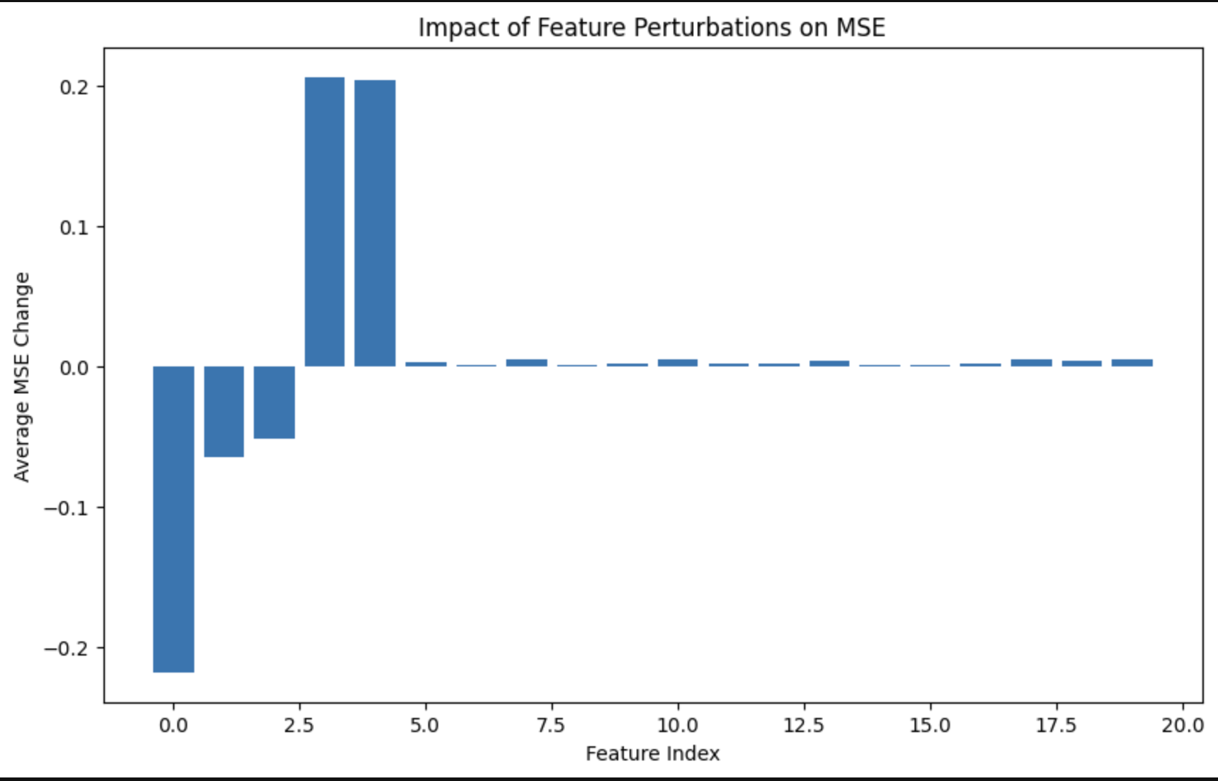
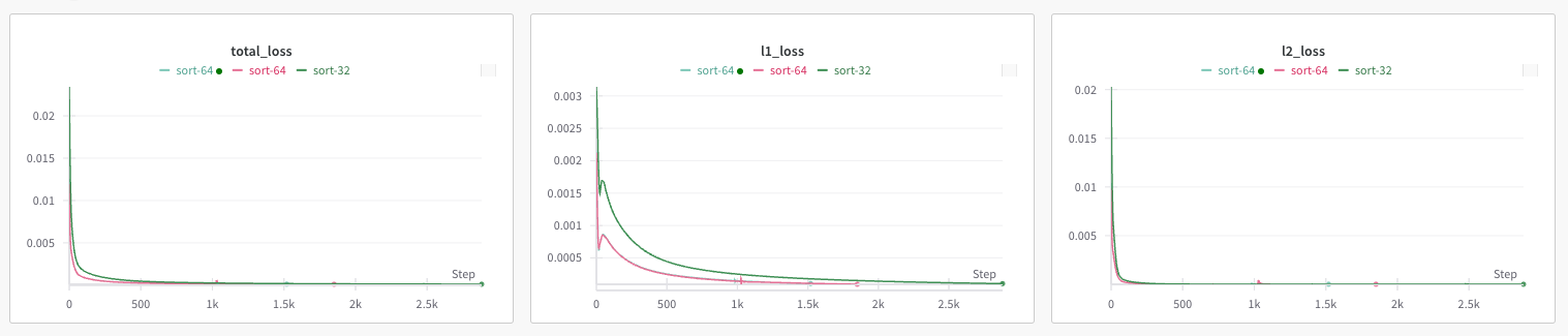
Here's some graphs from the toy model experiment I'm cooking up.

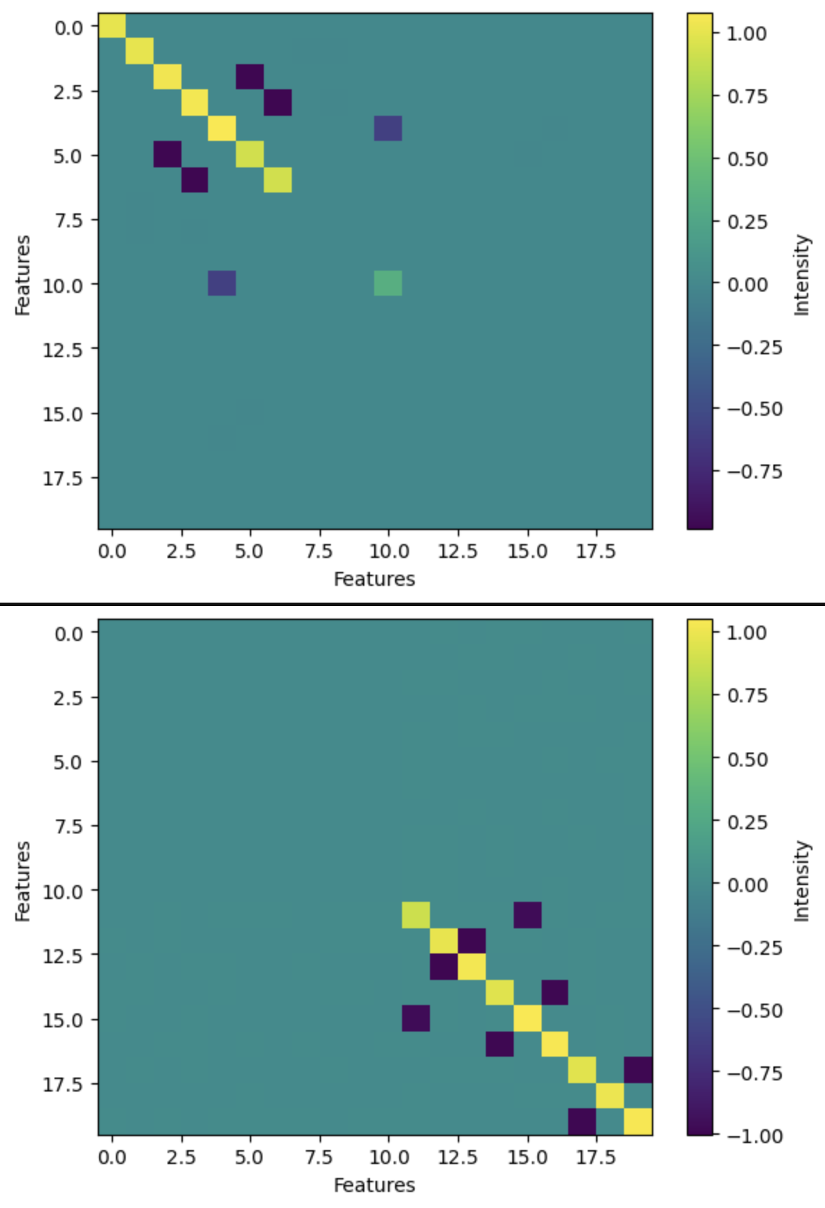
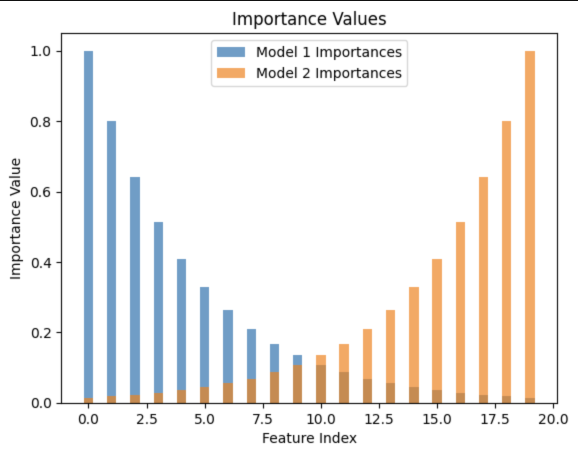
5:22 -> just spent like two hours 'fixing' what I thought was a bug, turns out it is not a bug.

guess which features are in superposition!